


Climate.gov brings us this guest post by Ken Takahashi, who is a research scientist at the Instituto Geofísico del Perú (IGP) and currently leads the national scientific committee ENFEN, which issues the official El Niño forecasts in Peru. This post does not necessarily reflect the views of IGP, ENFEN or NOAA.
El Niño was first identified by fisherman in the late 19th century off the coasts of Peru and Ecuador (Carranza, 1892; Carrillo, 1893). Unusually high Pacific Ocean temperatures depressed the region’s fisheries, and intense rainfall led to coastal flooding. The most extreme El Niño events, in terms of the surface warming in the eastern and central Pacific, occurred during 1982-1983 and 1997-1998. During these two events, Piura, a city in the coastal desert in northern Peru, experienced annual rainfall amounts equivalent to the other 40 rainiest years combined! The economic loss due to extreme weather in Peru during those events is estimated as 7% and 4.5% of its GDP, respectively (CAF, 2000).
The desire to help society prepare for those kinds of disruptions has led to great scientific advances in understanding El Niño. Still, one of the most frustrating things about El Niño for forecasters is why it doesn’t have the same impacts in the same places every time. In the past decade, the scientific community began to focus research on the diversity or flavors of El Niño and La Niña (the cold phase) as a possible explanation for the variability of impacts.
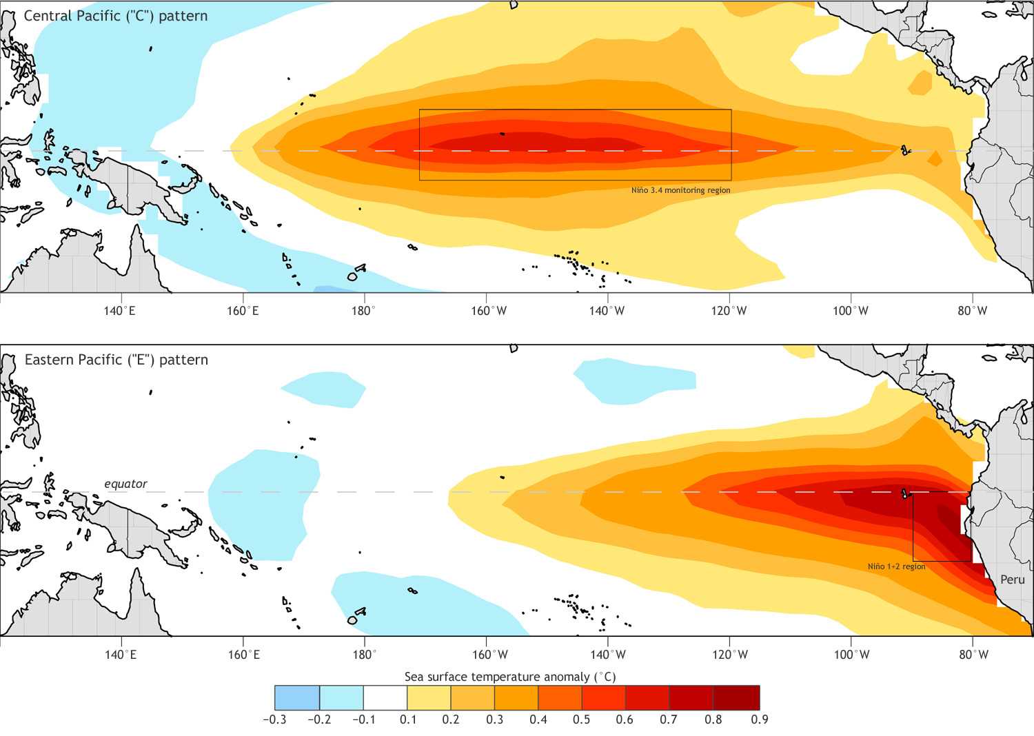
Pattern of sea surface temperature deviation from average (°C) associated with a unit value of the C index (top) and the E index (bottom), based on Takahashi et al., 2011. The Niño 3.4 and 1+2 regions are indicated as dashed boxes. Most El Niño events can be described as a combination of these two patterns. Image from Ken Takahashi.
Also Read: Who Will Get Snow This Winter If There Is A Strong El Nino?
In particular, they’ve focused on where along the equator the surface warming is largest, which does affect how El Niño and La Niña impact the global climate (Larkin & Harrison, 2005). Especially in Peru, El Niño can lead to very different rainfall impacts depending on whether the warming occurs in the eastern (wetter) or central Pacific (drier) (Lavado-Casimiro & Espinoza, 2014).
There are many different ways of classifying El Niño, but it is most common to measure it using sea surface temperature (SST) anomalies (departures from average conditions). In order to classify the different types of El Niño, however, we need at least two indices or time series (Trenberth and Stepaniak, 2001). Some colleagues and I introduced an E index and a C index(data here), which isolate the SST changes in the Eastern and Central Pacific, respectively, that are unique to each region (Takahashi et al, 2011).
How different are the extreme El Niño events from the regular ones?
Usually the SST warming in the central and eastern Pacific overlap, or correlate, during El Niño. But during the two “extreme” El Niño events (1997-98 and 1982-83), the warming in the east, near the coast of South America was much stronger than the warming farther west in the central Pacific (as can be seen in the left panel below).
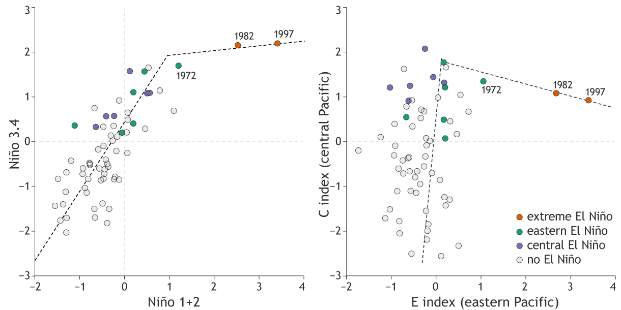
December-February average eastern and central Pacific sea surface temperature deviations from average: (left) Niño 1+2 (east Pacific; on x-axis) and Niño 3.4 (central Pacific; on y-axis); and (right): E (east Pacific; x-axis) and C (central Pacific; y-axis) departures from average. The year corresponding to December is indicated. Extraordinary El Niño events are indicated in red, while other eastern Pacific and central Pacific El Niño events are in green and blue, respectively. Gray indicates non-El Niño years. In both graphs, the dotted lines are an attempt to summarize the relationships shown by the dots, and the abrupt change of the slope of the dotted line highlights the uniquely different behavior shown by the 1982 and 1997 cases, and to a much smaller extent the 1972 case.
In fact, the values of the central Pacific Niño 3.4 index were only slightly greater than those of the 1972-1973 event, but the values were around 3 times greater in the eastern Pacific Niño 1+2 region. These geographic differences are also clearly depicted using the E and C indices (right panel), with very high E values during the two extreme El Niño events. This difference in central versus eastern Pacific warming during extreme events compared to regular ones is also evident in monthly C and E index values (see graphs below).
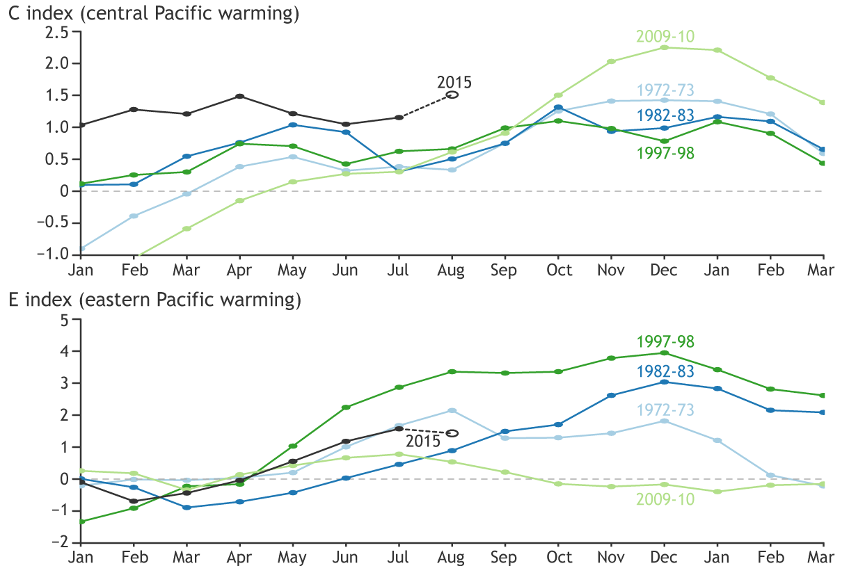
(top) Central Pacific (C) and (bottom) eastern Pacific (E) monthly SST indices during selected El Niño events and the current year. The estimated values for August 1-19, 2015, are indicated with an open circle. Graph by Ken Takahashi.
We found that this is because, once the normally cooler eastern Pacific warms enough for heavy precipitating storms, El Niño shifts to a faster gear: the Walker circulation shifts dramatically towards the eastern Pacific and the processes that lead to El Niño growth strengthen threefold (Takahashi & Dewitte, 2015).
Predicting extreme El Niño this year
If the physics of extreme El Niño events are different, then they should sometimes be analyzed separately from the rest; this also makes sense considering their large societal importance. Of great urgency this year: Are our scientific understanding and models good enough for the prediction of an extreme El Niño?
Although climate models provide objective predictions, models are far from perfect. They have common errors (particularly large in the eastern Pacific) and misrepresentation of slower changes in SST (decadal or 10-year timescales) or SST trends (2). By considering a collection of different models, or a multi-model ensemble (3), we hope that the errors cancel out among the different models. However, there are errors common to all models, such as the warm and rainy tendency in the cold and dry southeastern Pacific.
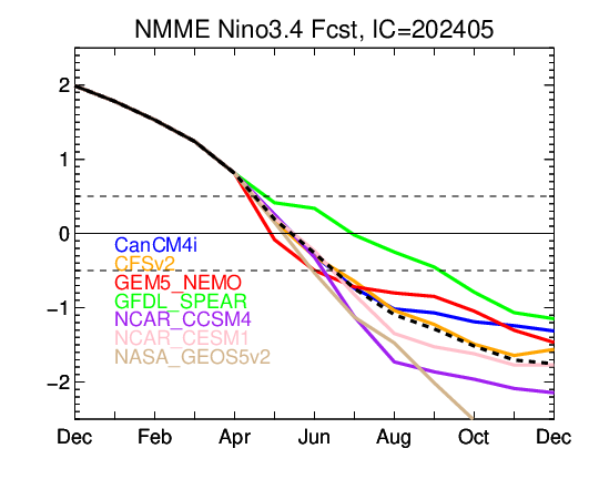
And we know that the models have a harder time making accurate predictions in the eastern Pacific. In particular, the models do not predict large enough SST anomalies in the far eastern Pacific during the extreme El Niño events (Takahashi et al, 2014). Even so, many models are predicting a strong El Niño in the central and eastern Pacific this year, similar to (or stronger than) 1972-1973, 1982-1983, and 1997-1998.
In addition to models, forecasters have other tools available, such as observational predictors and ideas based on physical common sense. The limitation in this case is the small number of events, with only two well-observed extremes, coupled with the fact that one El Niño is never a perfect mirror image of another El Niño, not even the extremes.
This year the ocean has accumulated a substantial amount of heat, a necessary condition for El Niño, but this does not tell us whether El Niño will be extreme or not in the eastern Pacific (Takahashi & Dewitte, 2015). Again, an extreme El Niño is a very different beast from the others in terms of impacts on weather and wildlife in the coastal regions of northern Peru and Ecuador, so El Niño strength is not just a detail.
One feature we found potentially useful is that if the trade (easterly) winds in the central Pacific become very weak around August, this allows the eastern Pacific to warm up a few months later, possibly enough to trigger strongly enhanced precipitation that could help El Niño become extreme (Takahashi & Dewitte, 2015). This did not happen in 1972, which is perhaps why that El Niño did not become as extreme.
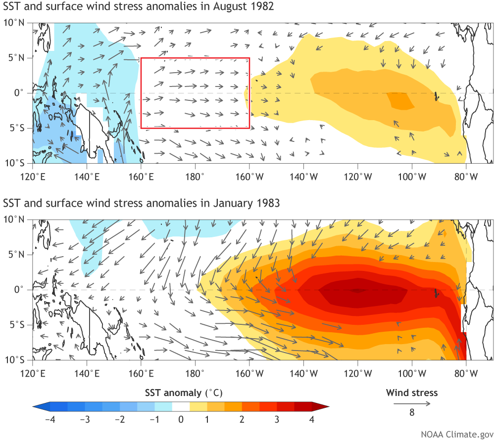
Difference from average sea surface temperature (colors) and difference from average of surface wind stress (arrows showing direction and strength by the length of the arrow line) in August 1982 (top) and January 1983 (bottom). The red box outlines the averaging region for the wind stress predictor for judging the probability of occurrence of an extreme condition in the Eastern Pacific 5 months later in January. Images adapted from Ken Takahashi.
This year we are putting this tool to the test. So far, the trade winds in August have not weakened as much as in 1997 but more than in 1982, indicating the probability of an extreme El Niño in 2015-2016. However, the eastern Pacific (E index) has been tracking the substantially weaker 1972 event and it would have to surge upwards, as in 1982, to become extreme (Fig. 3b). A quite different outcome could be that E keeps following 1972, remaining below the extreme threshold, while the central Pacific continues to warm into perhaps a larger version of the 2009-2010 El Niño (see bottom graph of Figure 3).
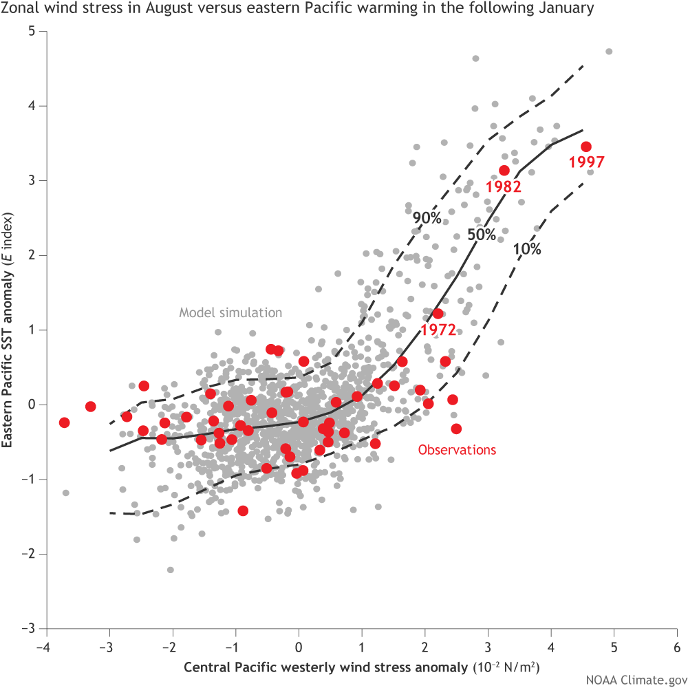
Predicted departure from average westerly wind stress (see footnote 1) in August (x-axis) vs. the eastern Pacific warming (E) in the following January (y-axis). Observations are in red, while the CM2.1 model ensemble forecasts (repeated model runs with different starting conditions) are grey, with their 10%, 50%, and 90% percentiles shown by the black sloping curves to summarize the positions of most of the gray dots. Adapted from Takahashi & Dewitte (2015).
As you can see, the chance of an extreme El Niño in the eastern Pacific is not straightforward to assess (5). Several factors will affect such a estimation. This year’s El Niño is already different from anything seen before. Furthermore, the rules of how the climate system works do not stay the same throughout time (e.g. climate change may affect El Niño), so statistical relationships found in a previous period might not be valid anymore.
Also, it is possible that random factors outside of the El Niño system could go against El Niño to keep it below the extreme threshold. Although several climate models are predicting a very strong El Niño, due to their common errors, we cannot fully trust them. Perhaps the only reliable rule is that El Niño can surprise us, and this year could be yet another example.
Anthony Barnston, lead reviewer
Footnotes
(1) The wind stress is based on the wind speed squared. Here, we are talking about the departure from average of the westerly wind stress. When the trades winds (winds from the east) become weaker, as they do during an El Niño event, the departure from average of the westerly wind becomes positive (because weaker trade winds mean stronger westerly winds, even if the actual wind is still from the east, but less strong than average). Then we square that departure from average. For example, if the westerly wind is usually -9 miles per hour, and now it is only -2 miles per hour, then the departure from average of the westerly wind is +7 miles per hour. And the departure from average of the westerly wind stress is the square of 7 miles per hour, which is 47 miles per hour.
(2) Changes in the entire North Pacific plus tropical Pacific on an approximately 10-year time scale, known as decadal variability, can change the backdrop behind El Niño and La Niña and encourage one of these at the expense of the other. As it turns out, much of the advances in El Niño science took place during a warm Pacific decadal phase, but we have been in a cold phase since approximately the year 1999 (although there are hints that we might be switching back to warm; we need to wait another year or two to make sure). Which decadal phase we are in can subtly, but noticeably, affect the strength of El Niño or La Niña, and our prediction models may not adequately take this decadal variability into account.
(3) A multi-model ensemble refers to the use of more than one model to make a forecast of deviations from average of climate or of sea surface temperature. Because each single model has its own biases or peculiarities, averaging the forecasts of several models tends to cancel these out and deliver a forecast having fewer specific biases. If several models have common biases, however, using more than one model does not help as much.
(4) The 1953-54 El Niño (leftmost green dot in both panels) had its largest warming in the eastern Pacific around mid-1953, but in DJF the eastern Pacific became relatively cool.
(5) Despite the large uncertainties in the eastern Pacific, Peru’s ENFEN will produce an estimate of the probabilities of the various strengths of El Niño, including the extreme type, later this week.
References
CAF, 2000: El Fenómeno El Niño 1997-1998. Memoria, Retos y Soluciones, V. Perú. Perú. Corporación Andina de Fomento, http://scioteca.caf.com/handle/123456789/676
Capotondi A, Wittenberg AT, Newman M, Lorenzo ED, Yu JY, Braconnot P, Cole P, Dewitte B, Giese B, Guilyardi E, Jin FF, Karnauskas K, Kirtman B, Lee T, Schneider N, Xue Y, Yeh SW, 2015: Understanding ENSO Diversity. Bull. Amer. Meteor. Soc., 96, 921–938, doi:10.1175/BAMS-D-13-00117.1
Carranza, 1892: Contra-corriente maritima, observada en Paita y Pacasmayo. Boletín de la Sociedad Geográfica de Lima, 1, 344-345.
Carrillo, C.N., 1893: Hidrografía oceánica. Boletín de la Sociedad Geográfica de Lima, 2, 72-110.
Larkin NK, Harrison DE, 2005: Global seasonal temperature and precipitation anomalies during El Niño autumn and winter. Geophys. Res. Lett., doi: 10.1029/2005GL022860
Lavado-Casimiro, W and Espinoza J.C., 2014: Impact of El Niño and La Niña events on rainfall in Peru (1965-2007). Revista Brasileira de Meteorologia, doi:10.1590/S0102-77862014000200003
Takahashi K, Montecinos A, Goubanova K, Dewitte B, 2011: ENSO regimes: Reinterpreting the canonical and Modoki El Niño. Geophys. Res. Lett., doi: 10.1029/2011GL047364
Takahashi, K., Dewitte, B, 2015: Strong and moderate nonlinear El Niño regimes. Climate Dynamics, doi: 10.1007/s00382-015-2665-3.
Takahashi, K., Martínez, R., Montecinos, A., Dewitte, B., Gutiérrez, D., Rodríguez-Rubio, E., (2014), White Paper #8a Regional applications of observations in the eastern Pacific: Western South America, Report of the Tropical Pacific Observing System 2020 Workshop (TPOS 2020), La Jolla, United States, 27-30 January 2014, GCOS report 184, vol. 2, 171-205.http://www.wmo.int/pages/prog/gcos/Publications/gcos-184_II.pdf
Trenberth, K. E., Stepaniak, D. P., 2001: Indices of El Niño evolution. J. Climate, doi:10.1175/1520-0442(2001)014<1697:LIOENO>2.0.CO;2