
 Images and Report From NOAA
Winter weather during the 2018 – 2019 season will be largely effected by the development of an El Niño trend. With NOAA predicting a 70% chance of an El Niño conditions for January, February and March the question turns to ‘how strong of an El Niño event are we in for?’
Note: During an El Niño, snowfall is greater than average across the southern Rockies and Sierra Nevada mountain range, and is well-below normal across the Upper Midwest and Great Lakes states.
The following report was made by Prof. Jason C. Furtado (@wxjay) of the University of Oklahoma School of Meteorology. His research group focuses on large-scale climate dynamics and applying that knowledge to subseasonal-to-seasonal forecasting, testing and evaluating operational and climate models, and future climate change.
In case you haven’t heard, there is now a 70% chance of an El Niño this winter. Having a confident prediction of El Niño this far ahead is quite a feat for the seasonal forecasting community. One reason ENSO is predictable six to nine months ahead of time is the North Pacific Oscillation (NPO) (1) and the related Pacific Meridional Mode (2). But, these precursors are unable to answer another critical question about El Niño: What will be the flavor of the El Niño event – i.e., a stronger, Eastern Pacific (EP) type (1997-1998 in example below) or a weaker, Central Pacific (CP) event (2004-2005 in example below) (3)? For that, I contend, you have to look to the South Pacific, a region that has received little attention in past ENSO studies. And the South Pacific suggests, if an El Niño forms this year, it will be a “weak” or CP event.
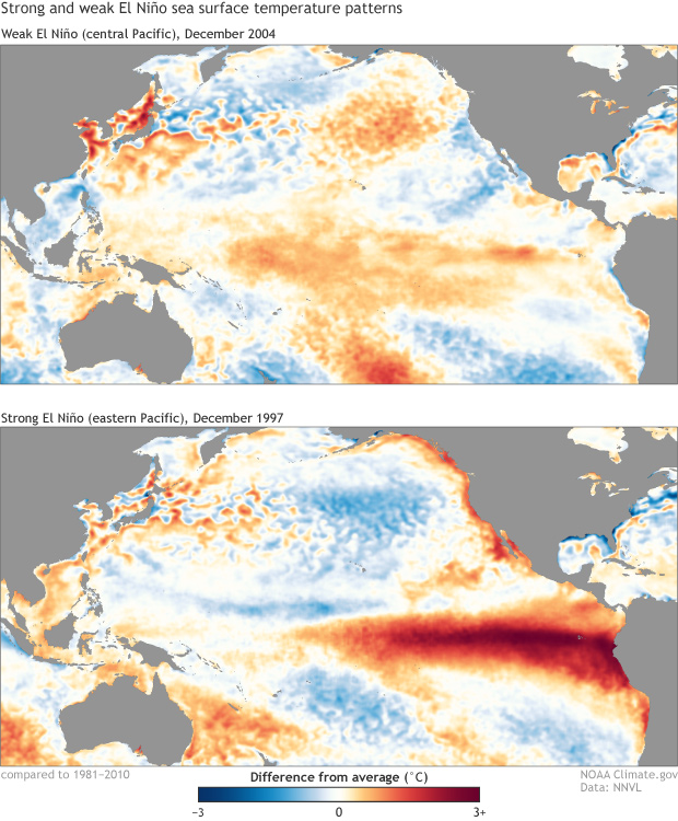
(top) Sea surface temperature anomalies derived from satellite during December 2004, a time when a weak El Niño event was present. Positive sea surface temperature anomalies were contained to the central Pacific. (bottom) Sea surface temperature anomalies derived from satellite during December 1997, a time when a strong El Niño event was present. Sea surface temperature anomalies are largest in the eastern Pacific and the positive anomalies extend from the central Pacific all the way to the eastern Pacific. Climate.gov image using data from the NOAAView.
But, before we get into the details, the term ‘flavors of El Niño” isn’t uniform throughout the climate community, and different definitions exist as to what an EP vs. CP El Niño event is. Indeed, ENSO is like many other elements of the climate system – it is not “this or that” but a spectrum of possibilities and outcomes. My colleague Michelle related different types of ENSO events to ice cream. Her conclusion on the matter is important: Weak El Niño events tend to have maximum sea surface temperature (SST) anomalies in the central tropical Pacific, while strong El Niño events tend to have their maximum SST anomalies in the eastern tropical Pacific. Therefore, I will use “strong/EP” and “weak/CP” in this post to ensure we understand what the event type means in terms of magnitude and location of the maximum SST anomaly. Keep in mind that many El Niño events cannot be clearly categorized and are a mixture of EP and CP. Also, while most EP events are stronger, full-basin El Niños there are some exceptions (like the coastal El Niño in 2017). In NOAA outlooks, the flavor of the event is implied by measurements of the strength of ENSO and the SST anomalies in different regions.
Introducing the South Pacific Oscillation
The first piece of the South Pacific – ENSO puzzle involves a newly identified pattern of variability in the South Pacific. In a recent study, we have identified the most commonly occurring pattern of sea level pressure (SLP) variations (5) in the Southeast Pacific during austral (i.e., Southern Hemisphere) winter (i.e., June – August). This dipole pattern features opposing fluctuations of SLP in two north-south oriented “centers of action” located between about 60°S and 35°S. We call this dipole the South Pacific Oscillation (SPO).

The sea surface temperature anomalies (SST) (shaded contours), 10-m wind anomalies (vectors), and sea level pressure (SLP) anomalies (line contours) associated with the South Pacific Oscillation (SPO). Positive (negative) values of SLP anomalies denoted by red (blue) solid (dashed) contours. Warmer than average SST are in yellows and reds while colder than average SSTs are in blues. Climate.gov animation using SST data from HadISST, and SLP data from NCEP/NCAR reanalysis.
The two centers of the SPO represent different physical processes in the Southern Hemisphere climate system. For this post, we will focus on the northern node of the SPO (i.e., the one off the west coast of South America). Physically, this “center of action” represents changes in the strength of the South Pacific subtropical high, a semi-permanent area of high pressure in the South Pacific. This high pressure center provides much of western South America (e.g., Peru and Chile) with a mild and relatively dry climate, much like the climate of coastal California (which – you guessed it – is also controlled by a subtropical high).
The negative departures from average (dashed blue contours in the image above) indicate a weaker-than-normal subtropical high, meaning a slackening of the climatological southeasterly trade winds. Therefore, upwelling, the bringing up of cooler water at depth in the ocean, is also reduced in the tropical Pacific, and warmer-than-average SSTs appear (shaded contours in the image above). Indeed, the SPO is well correlated with tropical Pacific SST anomalies, which is the first clue that this pattern is important for ENSO development. The SPO is most active during the winter months, which for the Southern Hemisphere is June – August (JJA).
The SPO as a Player in ENSO Development
Now let’s consider the evolution and development of an El Niño event. In June when an El Niño event is developing, warm water anomalies are already present in the central tropical Pacific. For development to continue, those warm central tropical Pacific SSTs have to build eastward and amplify during Northern Hemisphere summer and early fall (6). This eastward propagation of anomalies is driven by westerly winds and the formation of Kelvin waves in the ocean in the eastern tropical Pacific, thus allowing waters to get warmer there.
This process is actually a little easier said than done, and it is here that the SPO works its influence.
Since the SPO modulates the strength of the South Pacific trade winds in the eastern tropical Pacific, and it is most active during JJA, the phase and magnitude of the SPO can either help or hurt those Kelvin waves and the winds during the critical growth phase for ENSO. If the SPO is in the positive phase (i.e., a weaker South Pacific subtropical high), then the southeasterly trade winds weaken, which reduces the cold-water upwelling in the eastern tropical Pacific and allows for easier eastward propagation of the warm waters from the central tropical Pacific to the eastern tropical Pacific.
However, if the SPO is in the negative phase (i.e., a stronger South Pacific subtropical high), then the southeasterly trade winds intensify, and the cold-water upwelling in the eastern tropical Pacific also increases. These two factors create an environment hostile for eastward expansion of the warm waters. Thus, the warm SST anomalies tend to remain in the central tropical Pacific.
Putting it altogether: The SPO acts as an arbiter for where the maximum anomaly for the upcoming El Niño event will be located – i.e., the flavor of the event (7). That is:
- A strongly positive SPO during JJA means that the event will likely be a strong/EP El Niño.
- A near-neutral or negative SPO during JJA means that the event will likely be a weak/CP El Niño.
It’s Test Time
Let’s test these findings with real world forecasting applications. First, we identified all El Niño events (regardless of flavor) from 1950-present and then examined what the magnitude and sign of the JJA SPO was for that year. Using only that information, we predicted what the flavor of that El Niño event would be the following winter (8). The results indicate that our simple prediction scheme correctly predicted the flavor of the event nearly 3 out of 4 times. So it correctly predicted the strong/EP El Niño events of 1982 and 1997 as well as the two recent weak/CP ENSO events (2009-10 and the complex 2014-15 event). Of course, this scheme isn’t perfect (e.g., 2015), and more complex dynamics are certainly in play when looking at El Niño event evolution. But, the identification of the SPO and its important role in tropical Pacific climate dynamics is a key step forward (9).

The weekly average sea surface temperature (SST) anomalies (°C) for the week ending 21 July 2018 are shaded where warmer than average waters are in red and cooler than average are in blue. The average sea level pressure (SLP) anomaly (hPa) for the period 1 June 2018 – 19 July 2018 are in contours where dashed contours reflect lower than average SLP and solid contours represent higher than average SLP. The SLP anomaly pattern resembles a negative South Pacific Oscillation pattern. SST data from NOAA OI SST. SLP data from NCEP/NCAR reanalysis.
To Boldly Predict the Upcoming ENSO Event Using the South Pacific
Let’s return to our currently evolving event. What does the SPO have to say about the expected flavor of this year’s El Niño event (10)? The figure above illustrates that the SST warming thus far over the eastern tropical Pacific is spotty with evidence of subsurface warming present. Note that south of the Equator, however, there is an expanse of quite cold waters. More importantly, the SLP pattern in the South Pacific resembles a negative SPO signature (11). Indeed, for June 2018, the SPO index was about -1.3 (12), and the SLP anomaly pattern in the South Pacific thus far for July also suggests a negative SPO value for the month. Without a substantial turnaround for the SPO in August, the JJA SPO for 2018 could turn out negative. Thus, based on what I argued above, if an El Niño event forms this upcoming winter, it will most likely be a weak/CP El Niño event. Luckily, I am not totally alone in this prediction. The latest forecast from the NMME models (below) hints at a weaker/CP El Niño event evolving this winter.

The latest forecast of sea surface temperature (SST) anomalies (°C) for October 2018 – December 2019 from the North American Multi-model Ensemble. Forecast from models initialized in July 2018. Climate.gov image using data from NOAA’s Climate Prediction Center.
Regardless of how this specific event works out, this work and ongoing work in my group highlights that the South Pacific may be an untapped region for clues in understanding and forecasting tropical Pacific climate variability. I look forward to more pioneers joining my colleagues and myself into this relatively new frontier in ENSO research.
(Lead editor: Tom Di Liberto)
Footnotes
(1) The North Pacific Oscillation (NPO) is essentially a dipole of opposing sea level pressure anomalies between roughly Alaska and just north of Hawaii. This pattern can go by other names; e.g., the East Pacific – North Pacific pattern, for which NOAA CPC maintains an index. Tomayto, tomahto.
(2) You can learn more about the (North) Pacific Meridional Mode and how it works to “charge” the central tropical Pacific Ocean for an El Niño event from the guest blog post by Dan Vimont from the University of Wisconsin. I am using the qualifier “North” here because, based on some subsequent research (perhaps in a future blog post!), I have tied the work presented here into understanding the dynamics of the South Pacific Meridional Mode.
(3) The label “Eastern Pacific (EP)” or “Central Pacific (CP)” refers to where the maximum positive SST anomaly will reside – i.e., in the easternmost tropical Pacific (close to South America) or in the central tropical Pacific (e.g., near the dateline). Keep in mind that there are many El Niño events that are not cleanly categorized into one category. There is a continuum of SST flavors, where EP and CP represent the extremes on either end.
(4) These results come from published work by my graduate student Yujia You (@you_yujia) and myself (You and Furtado 2017).
(5) The formal definition of the SPO is the leading empirical orthogonal function (EOF) of monthly-mean South Pacific SLP anomalies between 10°S–45°S, 160°W–70°W. This leading mode explains ~50% of the total variance of SLP anomalies in that region.
(6) This process is also called the Bjerknes feedback and it is a self-reinforcing (i.e., a positive feedback loop). In this case, stronger SST gradients between the central and eastern tropical Pacific, together with anomalous convection forced by the warmer SSTs, induces stronger zonal winds. These zonal winds help to propagate and amplify the underlying SST anomalies, further strengthening the SST gradient.
(7) We have shown that this framework for the SPO also works for La Niña events as well, but here we focus on El Niño events only for brevity.
(8) For the determination of EP vs. CP, we used the Yeh et al. (2009) methodology, though, the results are insensitive if using other methods. The classification is: If the Niño-3 (Niño-4) index is greater than 0.5°C for three consecutive months and larger than the Niño-4 (Niño-3) index during DJF, then the event is an EP (CP) event.
(9) Further work by my graduate student and I have linked the SPO as the driver of the South Pacific Meridional Mode, which is akin to the North Pacific Meridional Mode. Look for information on that in a future blog post (hopefully!) or an upcoming manuscript.
(10) To be fair, we cannot make an apples-to-apples comparison, as we are only midway through July and the prediction scheme described relies on June, July, and August values of the SPO. But, we will work with what we have.
(11) No, it’s not a perfect match to the pattern shown in the first figure, but rarely does nature produce such a perfect match!
(12) The monthly SPO index value is based on a standardized version of the index – i.e., the -1.3 value means “-1.3 standard deviations below the mean” or -1.3s. The base period for standardization is 1981-2010, in line with other NOAA standardized climate indices.